A fast approch to OpenDX

OpenDX is a powerfull (very powerfull) program to visualize 2-3D data. In the opensource community, it is the equivalent of "grace" (or xmgrace) for 1D data.

I was extremely frustrated the first time I tried to use it because of the way the documentation was written (no offense intended : I am gratefull !). As it is the custom in the open source, if you're not happy with what you get, instead of complaining to people who owe you nothing, do it yourself. And so, this is why you're reading these lines.

If you use grace for 1D data (i.e. y=f(x) ), you know how easy it is to get started. Just put some two columns formated data in a text file, say "test.dat", and then at the prompt, type

$ xmgrace  test.dat

and you have a mgnificent graph in a nice window before your eyes ! You can do much better later by playing around menus and reading the manual, but hey, at least you have something.

Well, OpenDX does not seem so simple : you have the visual editor, the data model, the transformators and animators and renderers and executions, ... where to start ? The point of what I am writing is to show you that in fact, OpenDX is as simple as grace, and you can get your data displayed in seconds. Once you get the basics, you can spend hours learning all the power of dx.

Let's generate some data.

dx knows about a lot of sophisticated data format like HDF and CDF. I don't know about you, but I don't use these formats. I have rather arrays of data (in ascii or binary) like

2	4	6
3.1	3	5.5
1	4.4	2

let's generate some bigger array. The C program enclosed here generates the function z=sin(6*Pi*(x^2+y^2)) for x and y between -0.5 and 0.5 on a 100x100 grid. Compile the program

$ gcc -o generate generate1.c -lm      (Comment/Explanation)

and execute

$ generate > test1.data     (Comment/Explanation)

Now you have in the ascii file "test1.dat" your 100x100 z data. If you don't like C, generate the file with whatever you have at hand : scilab, text editor(tedious!), mathlab,pascal ...

Getting the picture

dx can read your data in (nearly) all formats. Just describe your data to it by

$dx -prompter

You get the following window:

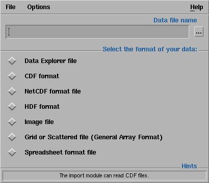
Put the name of your file ("test1.dat") in the "data file name" box and check the "Grid or Scattered file" box (your data is an evenly spaced grid). Your window enlarges to:

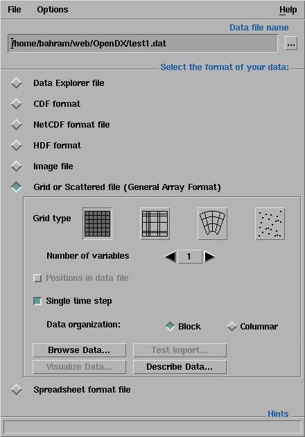
You get to describe your data by pushing the "describe data" button. A new and bigger window appears where you can put all the details about the way your data is organized :

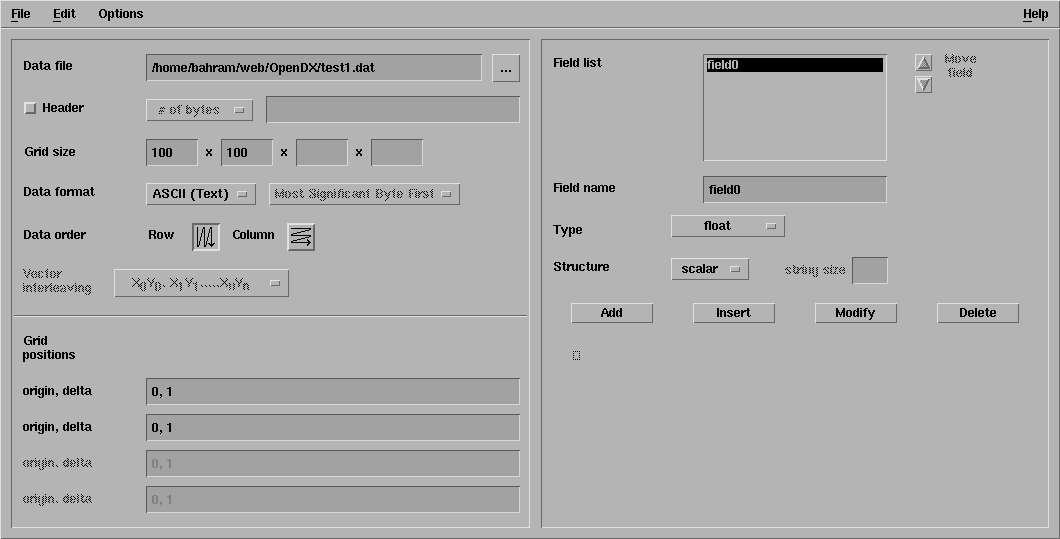
Your data here is simple enough and you don't have to give much details. The file name box is automatically filled ; The ascii menu is already chosen for "data format" ; the order doesn't really matter here. Just fill the Grid size boxes by putting 100 and 100 in it. Save the file as "test1.general" under the file menu. We'll get to this "test1.general" in a moment, but let's mention that it is a plain ascii file describing your data. Dx refers to this text file to read your data.
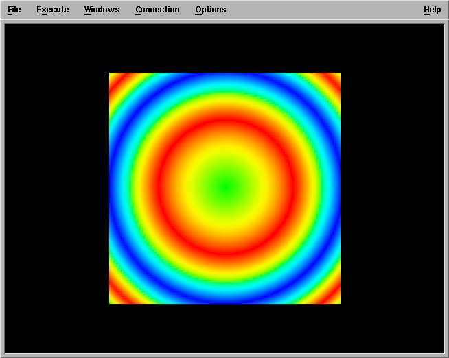
Now, close the description window and get back to the original data prompter window. As you can observe, the "visualize data" button is now active, so just push it. The graph appears in a new window :

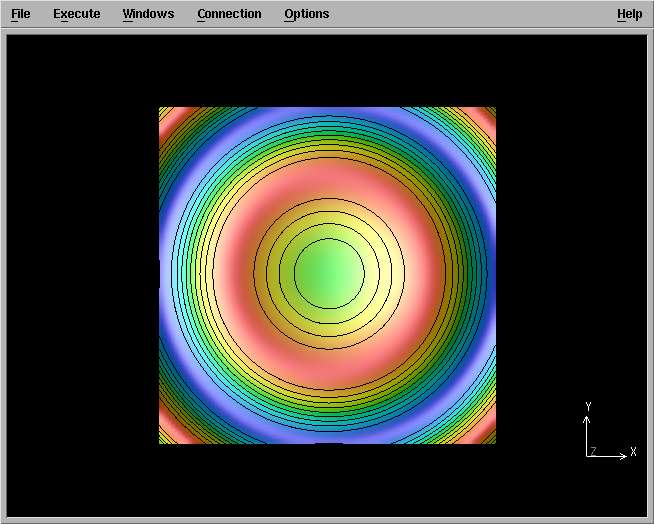
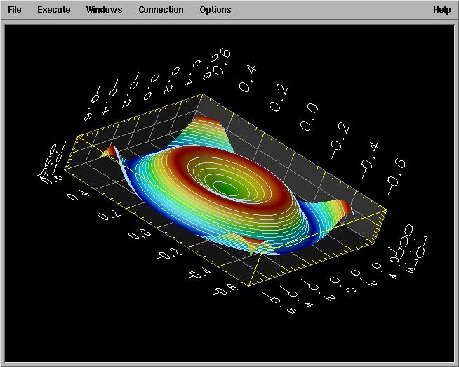
You can rotate the axes by dragging the mouse on the picture :

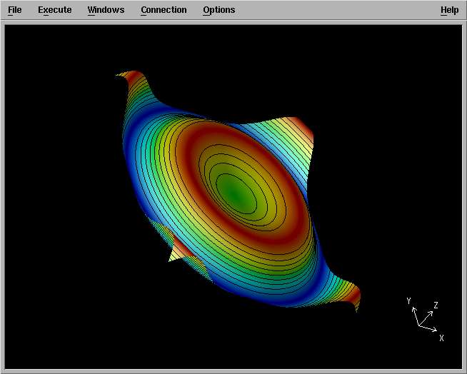
The Dx has chosen three diffrent kind of information to display : z-values are shown by both height and color code ; the countour curves (iso-z) are supperposed to the graph. You can explore the menus to zoom, navigate, rotate, change the color code,... Have fun.

A little more elaborate data

2 or 3D data are voluminous and seldom put in ascii files. Very often, they are in a binary format preceded by an N bytes header giving all kinds of useful information.

The "generate2.c" program enclosed here produce the same data as before, but put them in a binary format, preceded by 4100 bytes of information. By compiling and executing the program

 $ gcc -o generate generate2.c -lm
 $ generate

you get the test2.dat binary file described above. The data are in "double" format, which on my computer takes 8 bytes. The total file size is thus 100x100x8 + 4100 = 84100. Launching the data prompter

 $ dx -prompter

filling the "file name" box and pushing the "describe data" button get you again to the description window. This time, you have to give more informations :

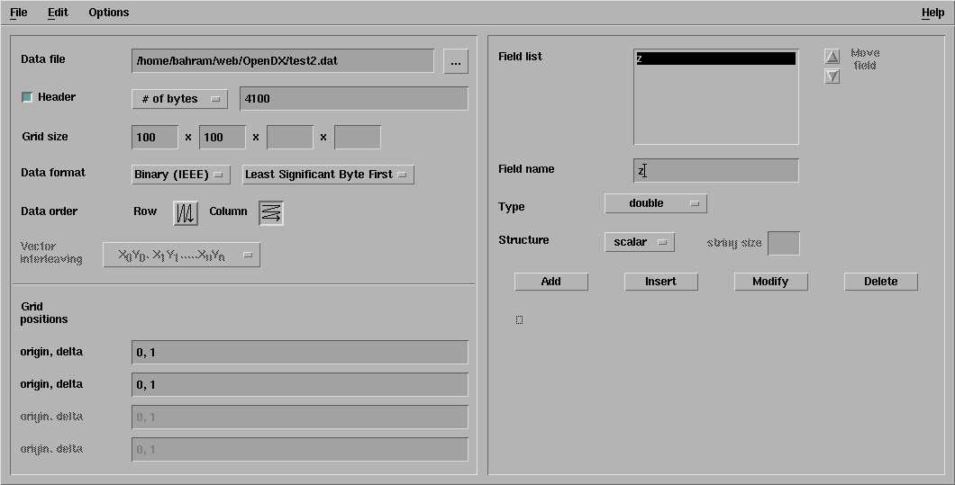
The header box has to be checked and #bytes put to 4100. That's the number of bytes dx will skip when reading the file.
Grid size is put as usual to 100,100
Data format is put to Binary(IEEE) with the "Least significant bytes first" option (on my computer)
Data order is put to Column (here the data are symetric and it does not matter, but in general, the order is critical)
The "type" (on the right) is put to double. Again, that's critical and dx has to know how many bytes it has to read per item.
you can give whatever name you want to the field (z here)
Don't forget to push the modify button to update the type change (dx is a little awkward here).

Saving the file under test2.general, closing the window and pushing the now active "visualize data" button give you the same image you had before.

Who needs the data prompter ?

Let's have a closer look at the "test1.general" file:

file = /home/bahram/web/OpenDX/test1.dat
grid = 100 x 100
format = ascii
interleaving = record
majority = row
field = field0
structure = scalar
type = float
dependency = positions
positions = regular, regular, 0, 1, 0, 1

end

That's a pretty "human" language to describe the data : the first line says where the actual data are, the second gives the grid size and so on. This is the kind of file we can produce easily with a text editor. So, quit all the "dx"es you have running. We'll suppose from now on that you possess a header file like the one above which describes your data file. When you pushed on the "visualize data" button, the data prompter in fact launched the "real" dx. Let us do it directly:

 $ dx -edit

This command gives you the "visual editor" window : a blank canvas on the right side and many (many many ...) items to choose from on the left side. Click on something on the left side, then click somewhere on the right side and you deposit the object on the canvas. Here, we have put three objects on the canvas :

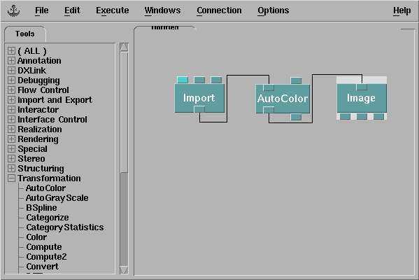
The first item is "import" from the "Import and Export" menu on the left side. This is to open and read the data file.
The last item is "image" from the "Rendering" menu. This is obviously to produce an image of the data.
The middle item here is "Autocolor" from "Transformation" menu. This is to tell the program which kind of information we need on the image. "Autocolor" associates colors to values, from blue to red as usual (of course, as everything in dx, this can be customized).

We have connected the ouput of "import" to the input of "Autocolor", and the output of this last one to the input of image. To connect objects, just drag the mouse from one output to an input.
We have to tell "import" where to import from. Double click on it, check the "name" box, fill the form with "test1.general" and click OK.

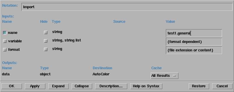
Now, from the menu "Execute", choose "Execute Once". Import will first read test1.general, learn how to read the real data in "test1.dat", read it and pass the information to "AutoColor". Autocolor will massage the data, produce colors accordingly and pass them to "image". This last one will display these colors on the screen :

The connected items you have on your canvas are called, in the IBM language, a "program". You can save them with .net extensions and call them directly from the prompt

$ dx -edit simple.net

if simple.net is the name you have choosed.
Change the middle object from "AutoColor" to "Transformation->AutoGrayScale" or "Realization->Isosurface" or "Realization->RubberSheet" to see some of the possibilities ( you have to "Execute->Ececute Once" each time to obtain the result.
A nice enough image of our data such as this

is obtained by this program

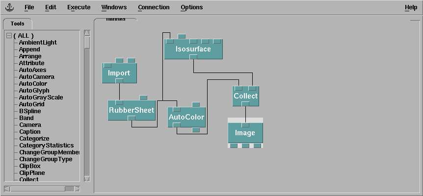
The data from "import" are first sent to "RubberSheet". This module converts the data you have to heights.
"RubberSheet" output is sent to AutoColor which as we said, associates color to values.
A copie of the "RubberSheet" output is sent to "IsoSurface". We have done a branching here.
The outputs of "Autocolor" and "IsoSurface" are merged together with "Collect" and sent to "Image".
Last thing, by modifying the options in the "Options" menu, we have turned on the axes and done some rotation for aesthetical purposes.

What's next ?

OpenDx can do much more than visualizing scalar data defined on a regular grid. The grid can be curvilinear, deformed or poorly defined, the data can have more than one dimension,... Think of visualising the deformation field of an engine complex part.
To go beyond this short introduction, You're on your own. The best sources of information are the manuals (quickstart, user's guide, reference manual ) given by the product, or downloadable at the official web site.
As a last thought, I think we can be gratefull to IBM. Whatever the reasons behind opensourcing DX (stabbing MS by pushing linux, too expensive to maintain,...) the product is just great. And then many thanks to the openpeople who continue to maintain and develop the Data eXplorer.

Up : various documents, mostly my lectures.
Next : Transifinite numbers (french)